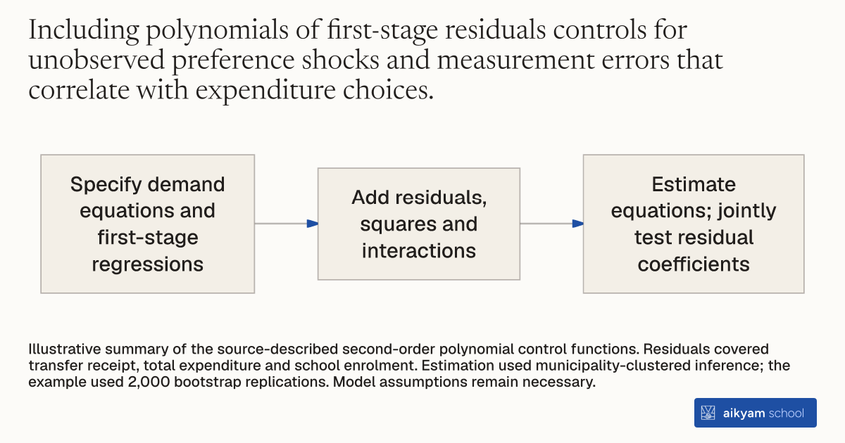
Research steps
Add control functions to demand equations
- Specify demand equations and first-stage regressions
- Add residuals, squares and interactions
- Estimate equations; jointly test residual coefficients
Illustrative summary of the source-described second-order polynomial control functions. Residuals covered transfer receipt, total expenditure and school enrolment. Estimation used municipality-clustered inference; the example used 2,000 bootstrap replications. Model assumptions remain necessary.
See source →How
When to use
Estimating how households change spending when given cash transfers requires controlling for total expenditure, schooling decisions, and program enrollment. Standard regressions fail because unobserved household preferences or measurement errors make these decisions endogenous. Adding flexible control functions isolates true changes in the intercept and slope of demand curves for poor welfare recipients.
Estimate household demand systems with non-linear endogenous regressors using a flexible second-order polynomial control function approach.
- Specify an Almost Ideal Demand System model relating budget shares to total expenditure, recipient gender, prices, and schooling choices.
- Estimate first-stage regressions for each endogenous variable using excluded instruments like wealth, firstborn gender, and municipality treatment status.
- Calculate the first-stage residuals for actual transfer receipt, total expenditure, and the number of children enrolled in school.
- Construct a second-order polynomial function containing the first-stage residuals, their squares, and their interaction terms.
- Add the polynomial function of residuals into the demand system equations as additional control variables.
- Estimate the demand system parameters using ordinary least squares or bootstrap methods clustered by municipality.
- Conduct a joint Wald test on all residual coefficients in the polynomial to check for endogeneity.
Why it works
Interacting residuals with endogenous variables allows researchers to identify changes in both the intercepts and slopes of Engel curves.
Example
Economists evaluated food budget shares for 811 households in Macedonia following a nationwide randomized cash transfer experiment. Using a second-order polynomial control function with 2000 bootstrap replications, researchers found that receiving a cash transfer targeted to mothers shifted the food Engel curve intercept up by 5.63 percentage points.
About the study
Participants
1053 households with children aged 14 to 18 sampled at baseline across 84 municipalities in Macedonia, with 830 households followed up after two years. Households averaged 4.5 members and 55 percent were Muslim.
Study Design
A randomized trial across all 84 municipalities in Macedonia, stratified by population size into 42 mother-recipient municipalities and 42 household-head-recipient municipalities. Surveys collected baseline data in 2010 and follow-up data in 2012.
Results
The control function estimate showed that targeting payments to mothers increased the food budget share intercept by 5.63 percentage points (p-value < 0.01). Within the food basket, mother-targeted transfers significantly steepened slope parameters for meat, fish, and dairy (-5.54) and salt and sugars (3.83).