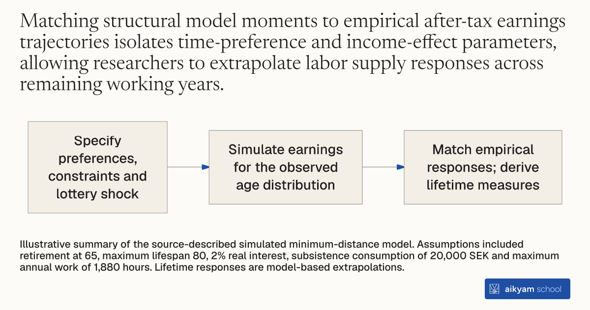
Research steps
Fit a life-cycle model to earnings responses
- Specify preferences, constraints and lottery shock
- Simulate earnings for the observed age distribution
- Match empirical responses; derive lifetime measures
Illustrative summary of the source-described simulated minimum-distance model. Assumptions included retirement at 65, maximum lifespan 80, 2% real interest, subsistence consumption of 20,000 SEK and maximum annual work of 1,880 hours. Lifetime responses are model-based extrapolations.
See source →How
When to use
Researchers need to extrapolate short-term empirical labor supply responses to estimate lifetime marginal propensities to earn and structural labor supply elasticities. Reduced-form estimates observe work adjustments over limited follow-up years, leaving long-term lifetime wealth effects unobserved. Estimating a dynamic life-cycle model using simulated minimum-distance matching aligns structural preference parameters with observed empirical after-tax earnings responses.
Fit a discrete-time dynamic life-cycle labor supply model with Stone-Geary preferences to empirical after-tax labor supply trajectories using simulated minimum-distance estimation.
- Specify a lifetime utility function over consumption and annual hours worked using Stone-Geary preferences with a binding retirement age at 65 and maximum lifespan of 80 years.
- Set fixed economic parameters, including a real interest rate r = 0.02, subsistence consumption gamma_c = 20,000 SEK, and maximum annual work hours gamma_h = 1,880.
- Treat the lottery prize as an unexpected exogenous shock to assets at the age of the winning event.
- Solve the agent's dynamic optimization problem to generate simulated post-lottery after-tax earnings trajectories across age cohorts matching the empirical lottery winner age distribution.
- Construct a minimum-distance criterion vector comparing simulated after-tax earnings responses to empirical reduced-form after-tax earnings estimates across follow-up years.
- Minimize the weighted distance criterion function to estimate structural parameters for consumption utility weight beta and discount rate delta.
- Compute implied lifetime marginal propensity to earn and labor supply elasticities (Marshallian, Hicksian, and Frisch) using the estimated preference parameters.
Example
Researchers matched a dynamic life-cycle model to 10-year after-tax earnings responses of Swedish lottery winners, estimating a consumption weight beta = 0.866 and discount rate delta = 0.014.
About the study
Participants
Simulated sample matching 244,826 observations of Swedish lottery winners aged 21 to 64 tracked over 10 post-win years.
Study Design
Simulated minimum-distance estimation matching 11 empirical moments to calibrate structural consumption weight and discount rate parameters in a dynamic Stone-Geary model with a 2% interest rate.
Results
The best-fit parameters yield a consumption weight beta = 0.866 and discount rate delta = 0.014 with chi-squared(8) = 3.385 (p = 0.092); implied lifetime marginal propensity to earn ranges from -0.169 at age 20 to -0.036 at age 60, with Marshallian elasticity = 0.010, Hicksian elasticity = 0.096, and Frisch elasticity = 0.150.