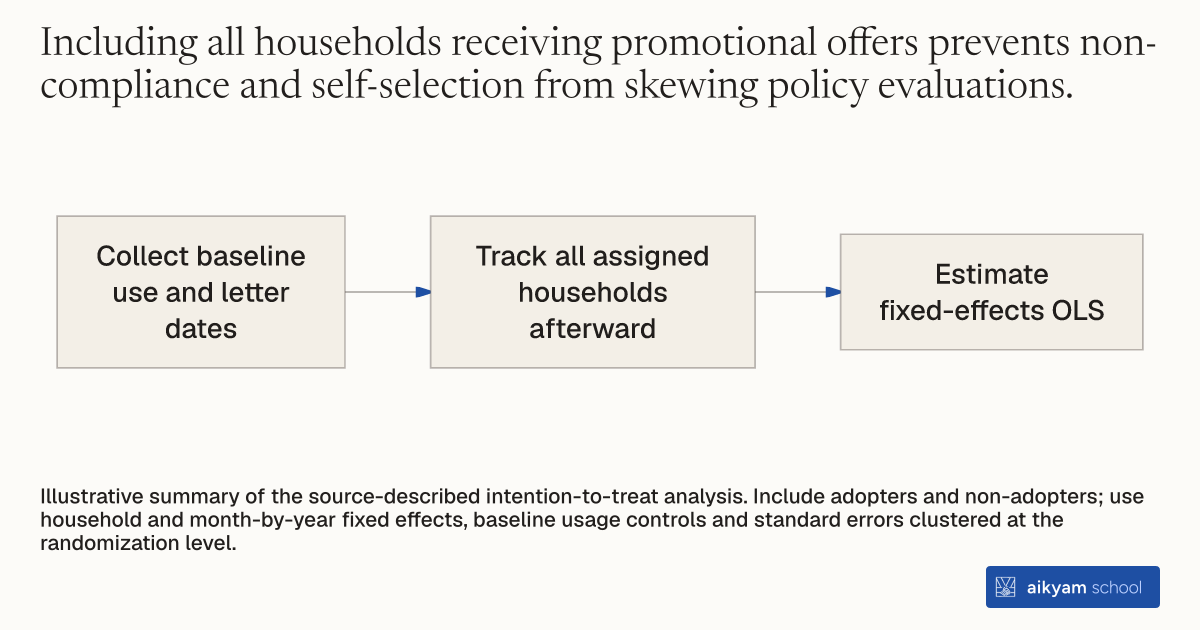
Research steps
Estimate the effect of outreach letters
- Collect baseline use and letter dates
- Track all assigned households afterward
- Estimate fixed-effects OLS
Illustrative summary of the source-described intention-to-treat analysis. Include adopters and non-adopters; use household and month-by-year fixed effects, baseline usage controls and standard errors clustered at the randomization level.
See source →How
When to use
Evaluating energy efficiency interventions requires analyzing full target populations regardless of compliance. Self-selection into technology adoption creates potential bias if non-adopters are omitted. Estimating intention-to-treat effects across all encouraged households measures the overall population-level impact of promotional campaigns.
Estimate the overall impact of sending promotional adoption letters on household monthly energy consumption using ordinary least squares with fixed effects.
- Collect baseline monthly energy consumption observations for all targeted households prior to intervention outreach.
- Record the calendar month in which promotional encouragement letters were delivered to each customer household.
- Track post-outreach monthly electricity and gas consumption across all assigned households regardless of whether they adopted smart meters.
- Specify an ordinary least squares regression model relating monthly energy use to an indicator variable switching to one after letter delivery.
- Include household fixed effects, calendar month-by-year fixed effects, and baseline usage controls in the regression model.
- Cluster standard errors over time at the randomization level to account for correlated consumption patterns.
Why it works
Fixed effects control for unobserved time-invariant household characteristics and seasonal weather fluctuations.
Example
Researchers evaluated monthly energy usage across nearly 40,000 British Gas households in the United Kingdom following promotional letter mailings, finding that letter assignment produced small, statistically non-significant changes in monthly electricity consumption ranging from -0.04 kWh to -0.15 kWh.
About the study
Participants
Nearly 40,000 residential British Gas households with 1,209,835 monthly electricity observations and 1,216,499 monthly gas observations in the United Kingdom.
Study Design
Ordinary least squares (OLS) intention-to-treat (ITT) regression analysis combining two experimental waves across six data-trimming specifications with household and month-of-sample fixed effects.
Results
Post-letter encouragement ITT coefficients for electricity were statistically non-significant across all six specifications, ranging between -0.04 kWh (SE 0.804) and -0.15 kWh (SE 0.871) per month relative to a control baseline mean of 296 kWh per month; gas ITT coefficients ranged from -0.15 kWh to +3.03 kWh per month (p > 0.1).