Research procedure
Estimate pricing effects on electricity use
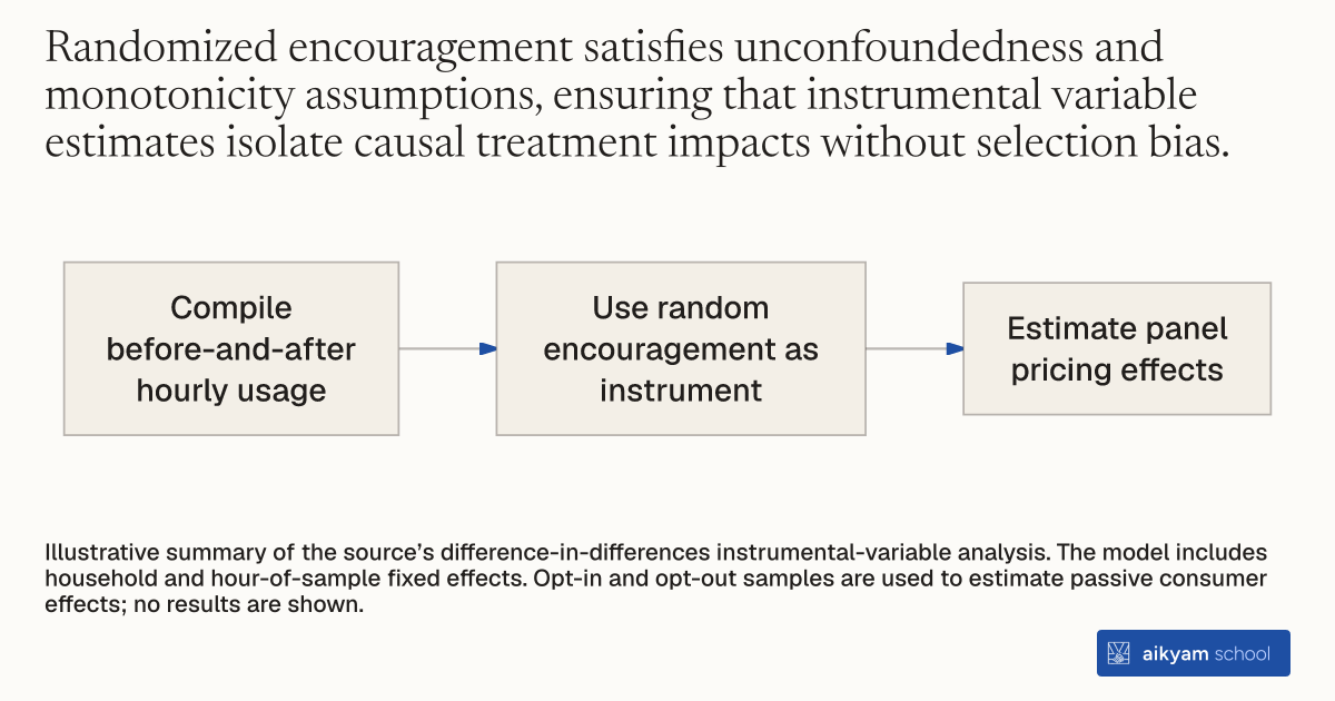
- Compile before-and-after hourly usage
- Use random encouragement as instrument
- Estimate panel pricing effects
Illustrative summary of the source’s difference-in-differences instrumental-variable analysis. The model includes household and hour-of-sample fixed effects. Opt-in and opt-out samples are used to estimate passive consumer effects; no results are shown.
See source →How
When to use
Program evaluators and energy economists need to measure the causal impact of dynamic pricing on electricity consumption across participant subgroups. Standard comparisons suffer from self-selection bias because voluntary joiners differ systematically from passive enrollees. Difference-in-differences instrumental variables estimation isolates local average treatment effects by using randomized encouragement assignments as instruments for actual program enrollment.
Estimate local average treatment effects of pricing tariffs on hourly electricity demand using two-stage least squares with randomized encouragement instruments.
- Econometricians compile hourly smart-meter electricity consumption data for treatment and control households across pre-treatment and post-treatment summer periods.
- Econometricians define an indicator variable equal to one during active treatment periods for households enrolled in time-varying pricing and zero otherwise.
- Econometricians instrument actual program enrollment using the randomized encouragement assignment indicator variable.
- Econometricians estimate a two-stage least squares panel regression model including household fixed effects and hour-of-sample fixed effects.
- Econometricians isolate passive consumer load reductions by running the two-stage least squares specification across opt-in and opt-out treatment samples using opt-out encouragement as the instrument.
Why it works
Panel fixed effects control for time-invariant household heterogeneity and hourly weather fluctuations.
Example
Researchers estimated peak electricity reductions across 174,000 residential households in Sacramento, California using DID-IV models, showing that Critical Peak Pricing reduced event peak load by 0.658 kW for active joiners and 0.242 kW for passive consumers.
About the study
Participants
46,684 CPP households and 48,245 TOU households evaluated across pre-treatment (2011) and post-treatment (2012–2013) summers in Sacramento, California.
Study Design
Panel Difference-in-Differences Two-Stage Least Squares (DID-2SLS) regression with household and hour-of-sample fixed effects, clustering standard errors by customer.
Results
Critical Peak Pricing enrollment reduced average hourly critical peak consumption by 0.658 kW per household for active opt-in joiners (p < 0.01) and 0.242 kW for passive opt-out enrollees (p < 0.01), while Time-of-Use enrollment reduced peak usage by 0.287 kW (p < 0.01) and 0.059 kW (p < 0.01) respectively.